

Phenomenology of Spatiotemporal Congestion Patterns
Three Ingredients to Make a Jam
The analysis of the complete image data base (check "any" in the input mask) suggests that there are three factors for traffic breakdown.
At first, we notice that nearly all traffic breakdowns occur at or near a bottleneck. In the images of the database, a bottleneck can be consituted by
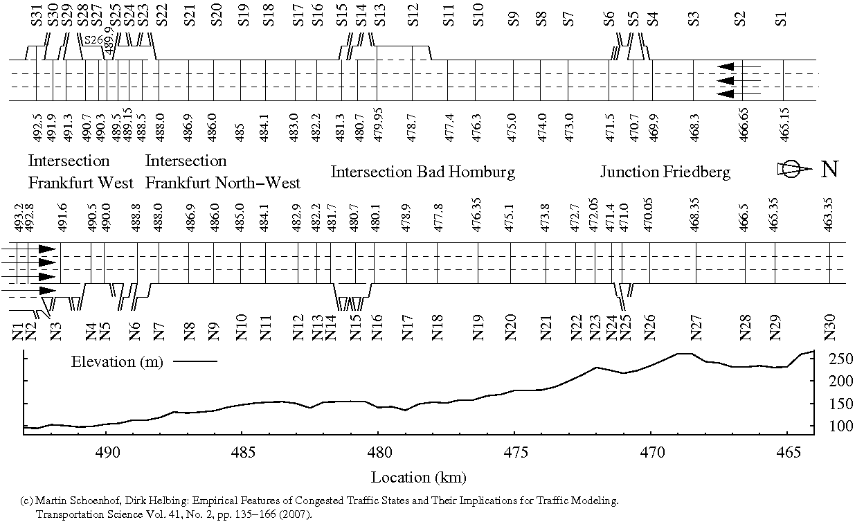
- Freeway intersections: "Westkreuz" near Kilometer 492, "Nordwestkreuz" at km 488, "Autobahnkreuz Bad Homburg" at km 480), see Sketch of the A5 section.
- Junctions: "AS Friedberg" at km 471.
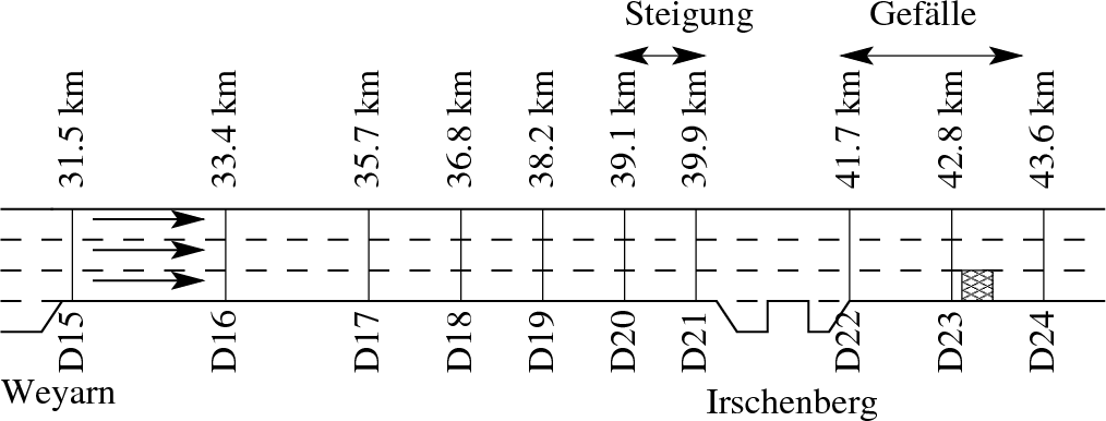
- Uphill and downhill grades: There is a significant uphill grade at the A5-North around kilometer 477-478. The corresponding downhill grade on the A5-South seems not to have a significant influence. Another infamous hilly section is the section "Irschenberg" on the German freeway A8-east, where similar congestions are observed.
- Accidents: At various locations. Enter "Accident" in the full-text string search to find instances in the image data base.
- Special cases: Examples are (moving bottlenecks) by heavy-duty special transports or median lawn mowing (enter "moving" in the full-text search), but also behaviour-induced bottlenecks such as "rubbernecking" when there is a spectacular accident in the opposite direction leading to a temporarily and locally less efficient driving style although there is no physical obstruction of any kind. (Unfortunately, we did not find conclusive examples in the image database. If you find one, we would be very happy to know)
Example of a traffic breakdown
Furthermore, as also suggested by common sense, a sufficiently
high traffic demand (in relation to the capacity) is necessary
for a traffic breakdown: Jams are rarely observed during the
small hours of the night although most bottlenecks are active during these periods
as well.
Finally, as third ingredient, one needs a final trigger in
form of an abrupt/inconsiderate driving maneuver provoking a
considerable perturbation. Trucks overtaking each other at small
speed differences ("running elephants") and the resulting
vehicle platoon can also serve as such a
final trigger.
These factors can be summarized by the three ingredients to make a jam (cf. the figure to the left ):
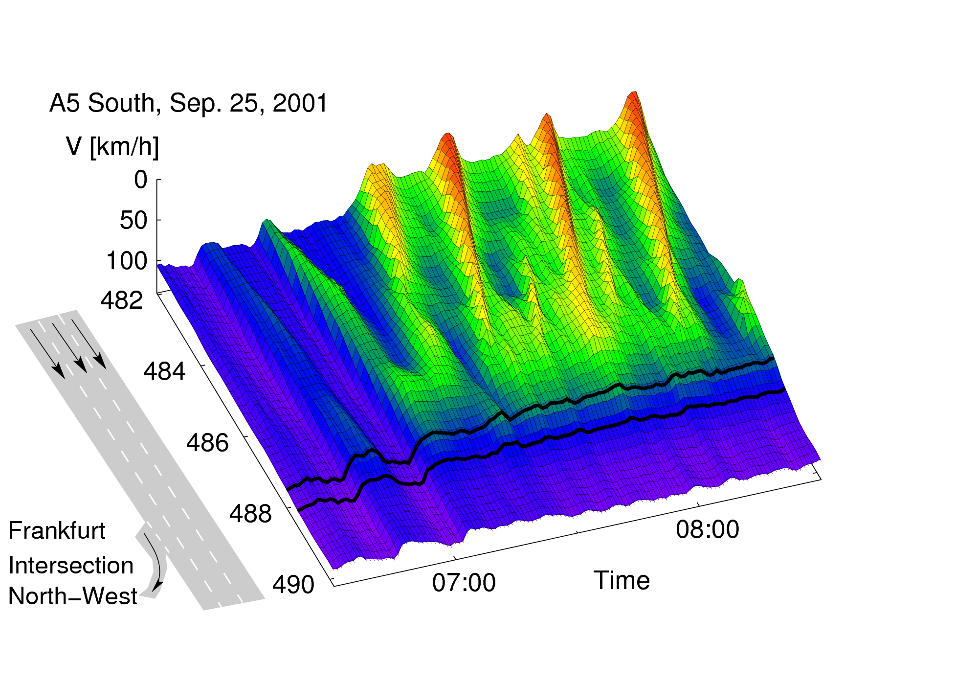
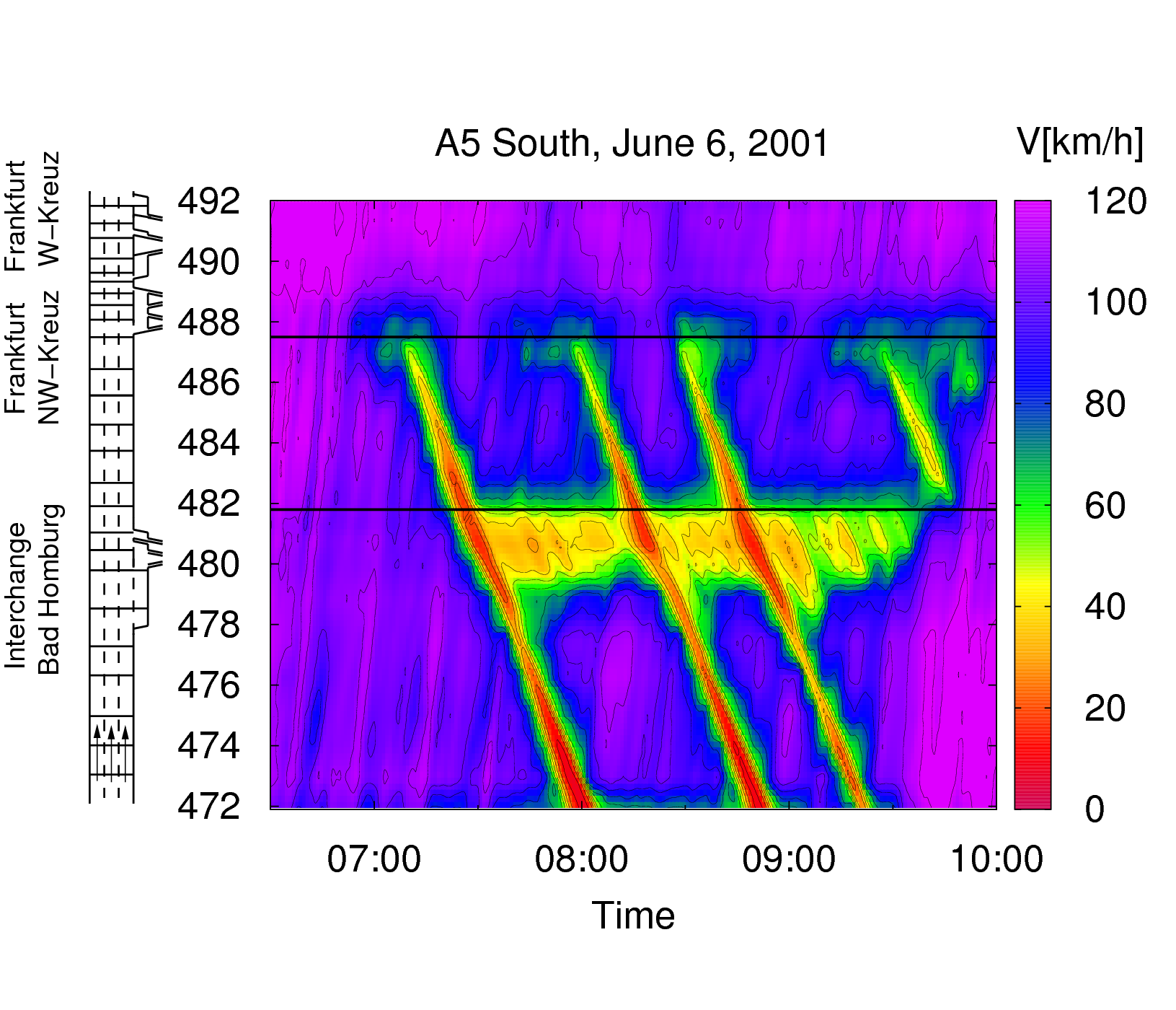
- High traffic demand. In the example depicted by the above image, this is the morning rush hour.
- Bottleneck. In this example, it is consituted by the exit ramps of the "Nordwestkreuz Frankfurt".
- Final trigger. Here, the triggering perturbation consists of a bounded region where the local speed drops to 80 km/h propagating at about the same speed.
In the example image above, there is evidence that the perturbation is caused by "running elephants" (trucks overtaking each other at slow speed difference): Due to the high traffic demand, a platoon of following vehicles forms behind the trucks. In the figure, this corresponds to a dark green spatiotemporal region (local speed about 80 km/h) propagating in driving direction with the cars (propagation velocity=local speed) at about 7:10 through the considered region. Further evidence for "running elephants" cause is given by the local traffic flow which is increased inside this region (not shown). As soon as the perturbation (the platoon) crosses the bottleneck, all three factors are true, and the actual breakdown (light green, yellow, and red regions) occurs at 7:10 near the road kilometer 488.
Qualitative Features of Jam Propagation: The "Stylized Facts
The images of the database as well as spatiotemporal patterns of jams of other traffic congestions on European and US freeways show remarkable similarities. On a qualitative level, they can be summarized by following rules, also known as stylized facts:
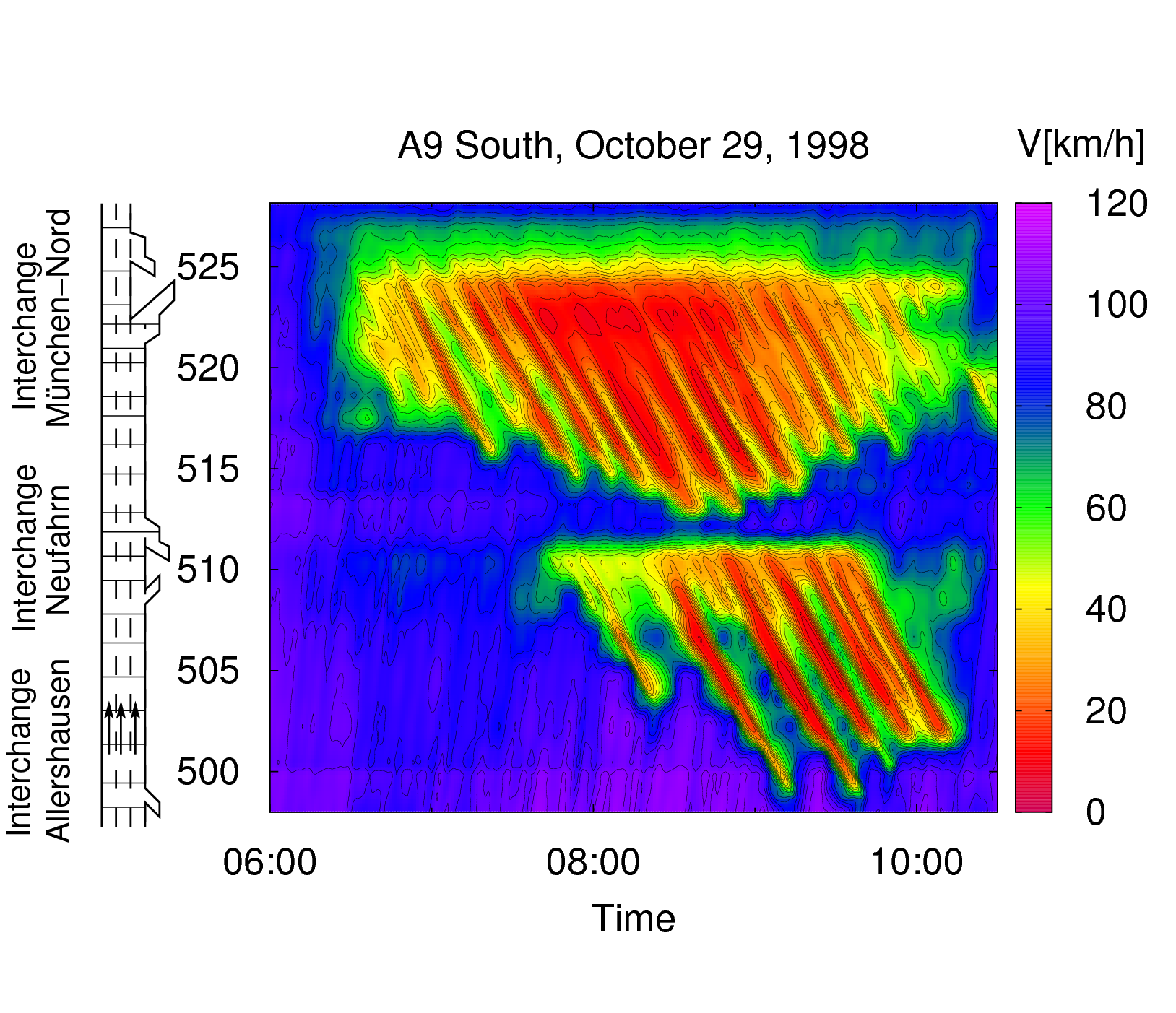
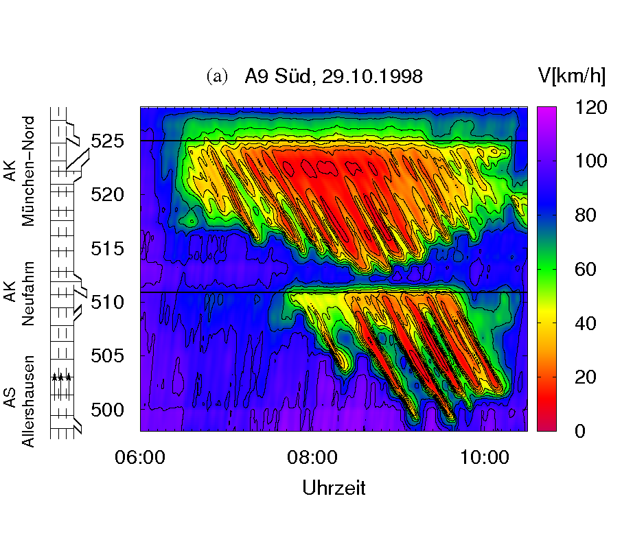
A9-South near Munich: Extended congestions behind two intersections
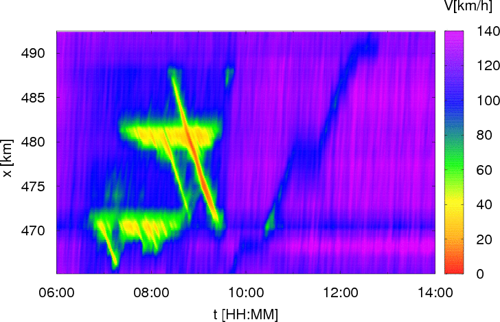
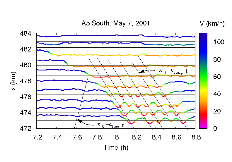
A5-South near Frankfurt: Localized stationary and moving jam waves
(1) Congestions may be localized (fixed spatial extension), or extended.
An extended congestion such as in the left image of the figure above has a variable spatial extension while localized congestions (or jam waves) such as these in the right image of the figure above, have a fixed spatial extension of typically 1 km.
(2) The downstream jam front is either stationary or moves with the characteristic constant speed c.
This is valid both for localized and extended congestions. In the case of localized congestions, one speaks of standing or moving traffic waves. In the case of extended congestions such as in this example from the freeway A9, the property of the downstream jam front can change abruptly from being stationary to moving (but not the other way round).
The propagation velocity c with values between -15 km/h und -20 km/h (depending on the driving style and vehicle composition but not on the congestion pattern) is the same as that of the position of starting vehicles in a queue of vehicles behind a traffic light. It corresponds also to the parameter ccong of the adaptive smoothing method used for generating the images.
(3) The upstream front of congestions is determined by supply and demand.

A8-East munich-Salzburg near the "Irschenberg"
The propagation velocity can be determined by making use of vehicle number conservation leading directly to the well-known shock-wave formula
| velocity of upstream front=difference of flow / difference of density |
between the regions of free and congested traffic separated by this boundary. From this and the above stylized facts it follows that this velocity is in the range between c (about -15 km/h) and the threshold speed Vc between free and congested traffic (about 45 km/h). Particularly, the velocity is positive (the congestion is shrinking) if the supply (i.e., the capacity at the bottleneck) is larger than the upstream traffic demand, see this figure after about 19:00. Otherwise, the velocity is negative (the congestion grows in upstream direction) as in the above figure before 19:00.
(4) The propagation velocity of perturbations/patterms inside extended jams is given by the constant value cc.
Nearly all extended congestions show internal oscillations or stop-and-go waves. With the exception of the upstream front itself (see Fact 3 above), the propagation velocity of all moving structures inside congestions moves at this speed. This includes moving downstream fronts (Fact 2). The analysis of microscopic traffic models such as the Intelligent Driver Model shows that this velocity can be expressed by
| c = -(vehicle length + minimum gap) / Net time gap in car-following mode, |
for example
| c = -(5 m + 2 m) / (1.4 s) = -5 m/s = -18 km/h. |
Of course, one must consider averages over the vehicle fleet and the different driving styles. Since the typical vehicle on US roads is longer compared to the typical European vehicle, the absolute value of c depends weakly on the country (typically, -18 km/h in the USA and -15 km/h in Europe).
(5) Oscillations inside extended congestions grow as they propagate.
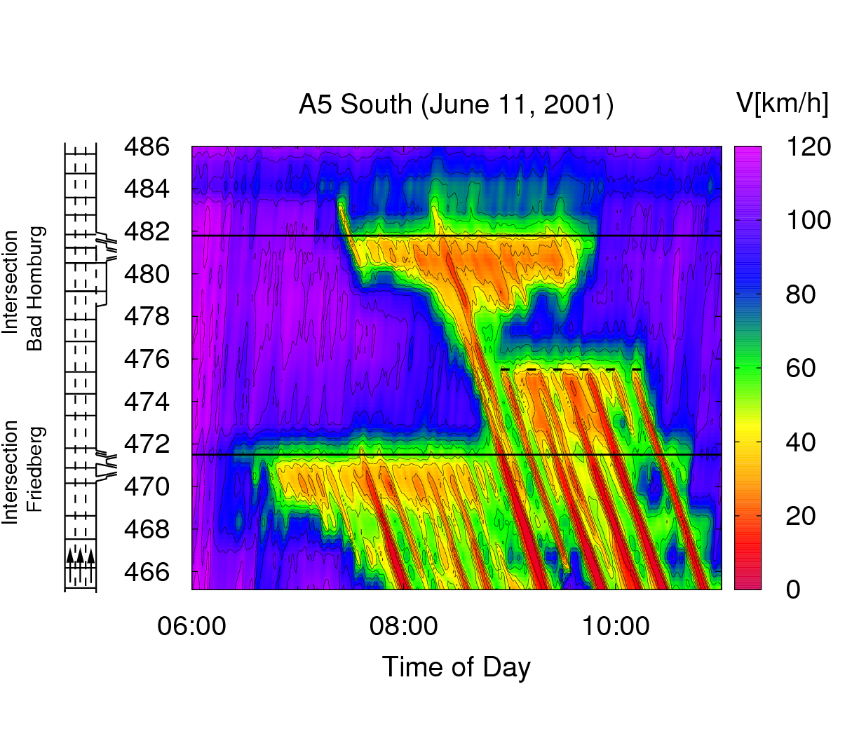
A5-South, congestions caused (from left to right) by a junction, an intersection, and an accident, respectively.
In most cases, congested traffic flow is essentially stationary near the downstream front (see the image to the left). However, during the course of time, small perturbations develop to traffic oscillations, and sometimes even to isolated traffic waves.
(6) The wavelength and period of the oscillations tends to decrease with the severity of the bottleneck.
This means that, in contrast to the propagation velocity, the wavelength is not a "traffic constant". The period varies between 4 min (severe congestions) and about 20 min (light congestions) corresponding to wavelengths between 1 km and 5 km, respectively.
For example, in this spatiotemporal speed profile of traffic on the A9, the intersection "Munich North" represents a more severe bottleneck compared to the intersection "Neufahrn", and correspondingly produces traffic waves of a higher frequency. The same applies to the complex composite congestion on the A8: The congestion caused by an accident contains traffic waves of a higher frequency compared to the congestions caused by the gradients of the "Irschenberg".
(7) Very weak or very strong bottlenecks may cause extended congestion without significant oscillations.
Enter "HST" (homogeneous synchronized traffic, light bottleneck), or "HCT" or "Accident" (homogeneous congested traffic, strong bottleneck) into the fulltext search and look at the results.
(8) Moving Bottlenecks.
Moving Bottleneck on the A5-North causing an extended congestion whose downstream front moves with the bottleneck
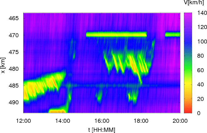
Moving Bottleneck on the A5-South causing no traffic breakdown
As all rules, also the Stylized Facts of Traffic Patterns have an exception. It is related to moving bottlenecks that may be caused, e.g., by special heavy transports, "running elephant" races of particularly slow trucks, or by moving road works such as mowing the median lawn. Enter the keyword "moving" in the search mask to see some examples. Such moving bottlenecks may cause congestions (see this example), or not, as in this example.
If congestions are caused, the moving downstream front violates Stylized Fact No. 2. However, this rule can be generalized to include moving bottlenecks:
(2a) The downstream front moves either with a velocity equal to that of the bottleneck, or with the velocity c
The other Stylized Facts remain unchanged. Note that the velocity of the bottleneck may be positive or negative.
By the way: For the case of moving bottlenecks, the distinction between Jam Ingredient No. 3 ("perturbations inside the traffic flow") and No. 1 ("bottleneck") smears out: "Running elephants" can be considered either as a moving bottleneck, or as a perturbation inside the flow. This ambiguity becomes irrelevant when defining two sets of "three ingredients": Either
| high demand+bottleneck+perturbation = breakdown |
or
| high demand+bottleneck + other crossing bottleneck = breakdown |
Quantitative Features
Time series of different detectors
For a
as a function of the bottleneck strength.
All four quantities (the features and the bottleneck strength itself) can be determined from the speed time series of several neighboring detector cross sections, at least indirectly.
Bottleneck strength
The bottleneck itself, definied as the degree of reduction of the
local capacity with respect to the neighboring sections,
cannot be determined directly. However, the bottleneck
strength is highly correlated witht he
Notice that, according to Stylized Fact No. 5, the speed variations at this location are small such that this instrument variable generally is well-defined.
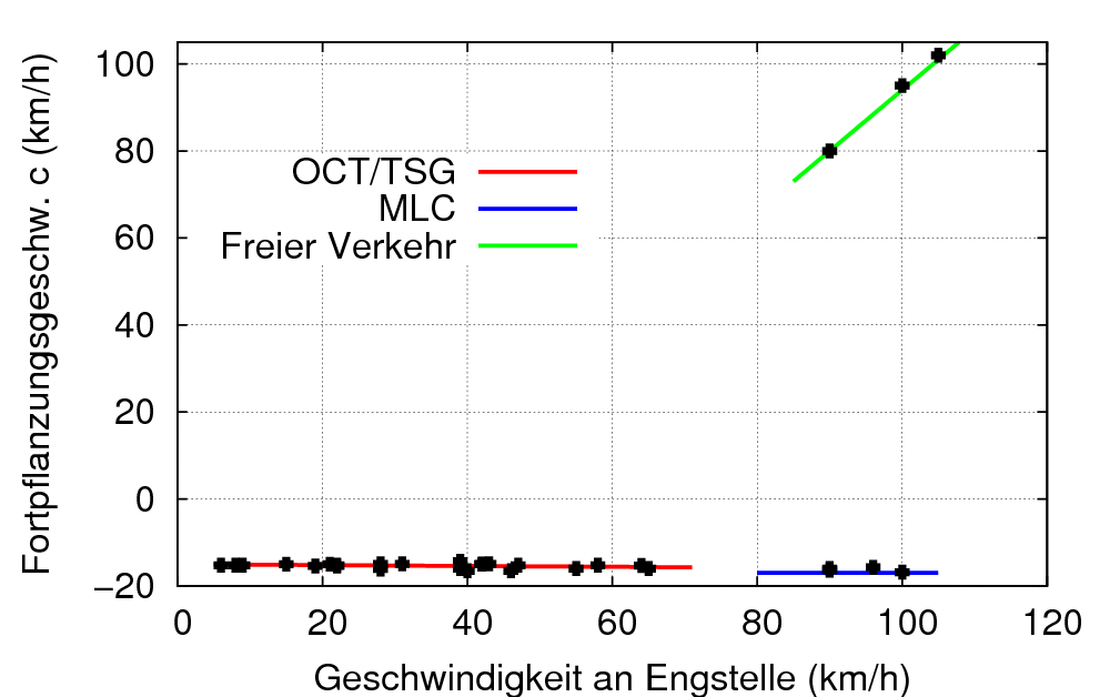
Propagation velocity
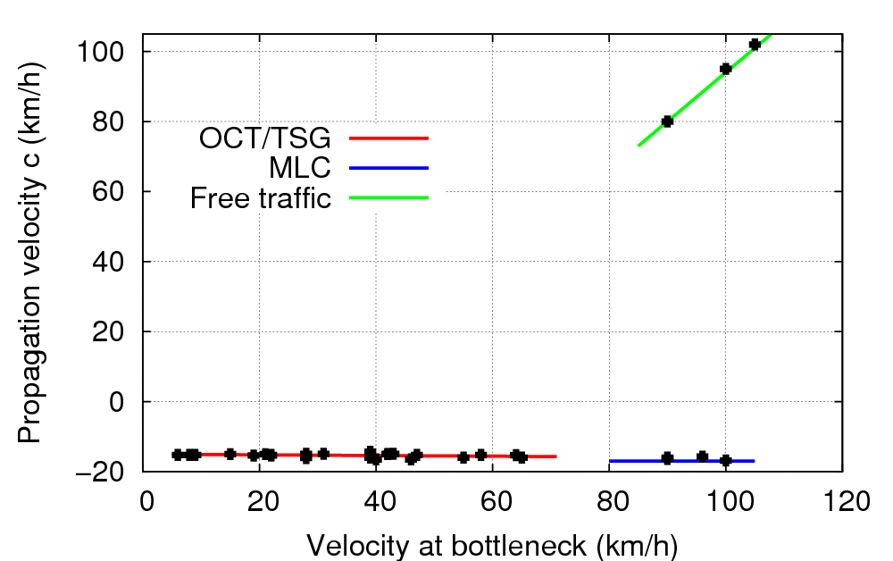
Propagation velocity of the traffic oscillations
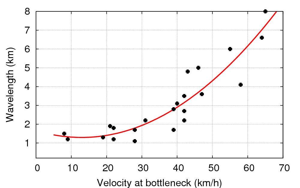
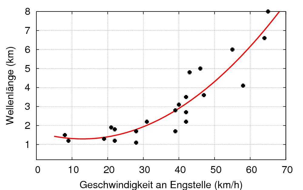
Wavelength of the traffic oscillations
From the time series, one obtains the propagation velocity by shifting the time series of adjacent detectors relative to each other until the first nontrivial peak of the correlation is obtained (of course, the trivial global maximum is obtained for a relative shift of zero). Then, the propagation velocity is simply given by detectors divided by
| propagation velocity c = τshift / (distance between detectors). |
An evaluation of the data behind the image data base resulted in remarkably constant values for c both for extended congestions (OCT and TSG) and moving localized jams (MLC). (Notice that all these abbreviations OCT,TSG, MLC are searchable by entering them in the full-text search mask of the image database.) This agrees with Stylized Fact No. 4.
Wavelength
One can read the average period directly from the speed time series of detetors where the traffic waves can be distinguished clearly from noise but are not yet saturated. In this figure, the suitable region is between the road kilometers 474 and 477. Using the propagation velocity c determined earlier, this also gives us the wavelength λ:
| Wavelength λ = |c| · τ |
A systematic evaluation of the data behind the images resulted in the depicted dependency of the wavelength with respect to the bottleneck strength: The wavelength reduces with the bottleneck strength (with reduced speed at the bottleneck) until a minimum value of about 1.5 km is reached for speeds smaller than about 25 km/h (to see some examples, enter "OCT" into the search mask). On the other hand, for very small bottleneck strengths, one obtains isolated traffic waves (enter "TSG" into the search mask) for which the definition of a wavelength no longer makes sense. All this is in agreement with Stylized Fact No. 6.
Growth rate
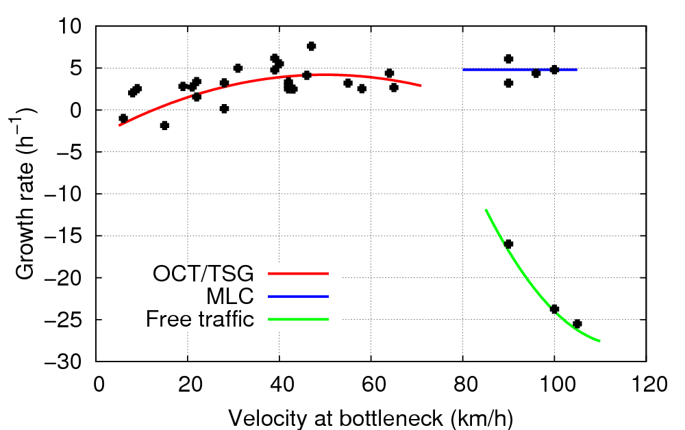
Growth rate of the traffic waves
Finally, one can determine the growth rate from the detector data. The spatiotemporal region to determine this quantity is the same as that for determining the wavelength, i.e., it should be possible to discriminate the oscillations from noise but they may not be saturated. Otherwise, the growth rate cannot be determined (only noise), or is biased to lower values (saturation). In our example, this is satisfied between the road kilometers 474 und 477. Sufficiently far away from the saturation, the growth rate is exponential, in a good approximation. This means, the average amplitude (of the speed oscillations) can be modelled by
| A = A0 · eσ(t-t0). |
By means of the time shifts τ already needed for calculating the propagation velocity, the growth rate σ can be determined by
| σ = 1/τshift · ln(Aup/Adown). |
The result agrees with the Stylized Facts Nr. 5 and 7: The growth rate of congested traffic is positive (growing waves) with the exception of very light or very severe congestions, and it is negative (traffic flow is stable with respect to perturbations) for free traffic. (However, negative growth rates cannot be determined with the method described above since no oscillations exist in this case; it has been determined differently.)
References
- Dirk Helbing, Martin Treiber, Arne Kesting, Martin Schönhof:
Theoretical vs. Empirical Classification and Prediction of Congested Traffic States,
The European Physical Journal B 69, 583-598 (2009).
Abstract,
Preprint.
- Martin Treiber, Arne Kesting, Dirk Helbing:
Three-phase traffic theory and two-phase models with a fundamental diagram in the light of empirical stylized facts,
Transportation Research Part B: Methodological 44(8-9), 983-1000 (2010).
Abstract,
Preprint.