

The Adaptive Smoothing Method (ASM)
Reconstructing the Spatiotemporal Speed Profile: Problem Statement
A detailled representation of the traffic situation in
space and time allows to analyze numerous aspects of traffic
dynamics and traffic theory. However, the commonly available
stationary detectors
only provide information at certain locations and at given time
instances (every minute, in our case), see the following
image on the
left.
The task of the reconstruction consists in estimating the values of
the local speed (or other traffic-related quantities) ;)
Aggregated speed data of stationary detectors
;)
Reconstructed spatiotemporal speed profile
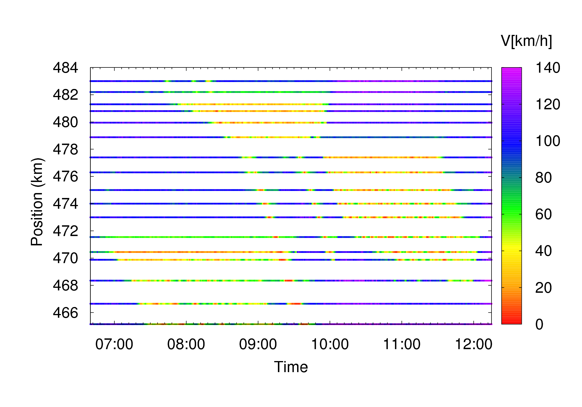
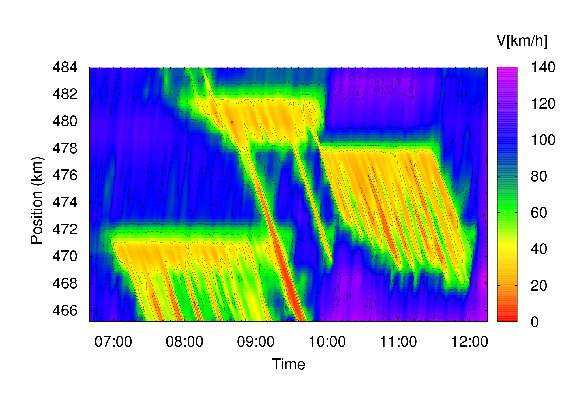
A simple independent local smoothing and interpolation (e.g., by separately applying moving averages in space and time, or by assuming the value of the data point which is nearest to the point (x,t) for which the speed should be determined) is not suited since the spacing between two neighboring detector stations is of the same order as the typical dimension of traffic patterns such as the wavelength of stop-and-go waves. Consequently, these simple methods lead to artifacts such as the checkerboard pattern of the image to the left. In contrast, the traffic-adaptive interpolation with the Adaptive Smoothing Method, ASM) takes care of dynamic invariants of the correlations of traffic patterns (constant propagation velocities of perturbations in free and congested traffic, see the Stylized Facts) leading to plausible results as shown in the right-hand image of the following figure).
;)
;)
Independent interpolation/smoothing of space and time leading to artifacts
;)
Interpolation/smoothing with the adaptive smoothing method
Specifically, this method makes use of the empirical observation that all macroscopic perturbations of traffic flow (such as changes of the local speed) either are stationary, or propagate with one of two characteristic velocities (see Stylized Facts):
- In free traffic flow, perturbations propagate essentially with the vehicles, i.e., the propagation velocity is equal to the local speed average.
- In congested traffic, perturbations propagate against the driving direction at a remarkably constant velocity of about -15 km/h.
The negative velocity of perturbations in congestions can be understood in terms of the driver reactions: Specifically, the absolute value of the velocity is essentially given by the average effective car length (car length + minimum gap in standing traffic) divided by the average time gap in car-following mode. This means, the velocity depends weakly on the average driving style and traffic composition but does not change with the type of congestion. Specifically, the same value applies for
- stop-and go waves,
- perturbations inside extended jams,
- moving downstream fronts of extended jams,
- location of the starting vehicles in a queue behind a traffic light after the light turned green.
The two nonzero propagation velocities for free and congested traffic are discriminated by a nonlinear speed filter (for details, see the references).
Parameters
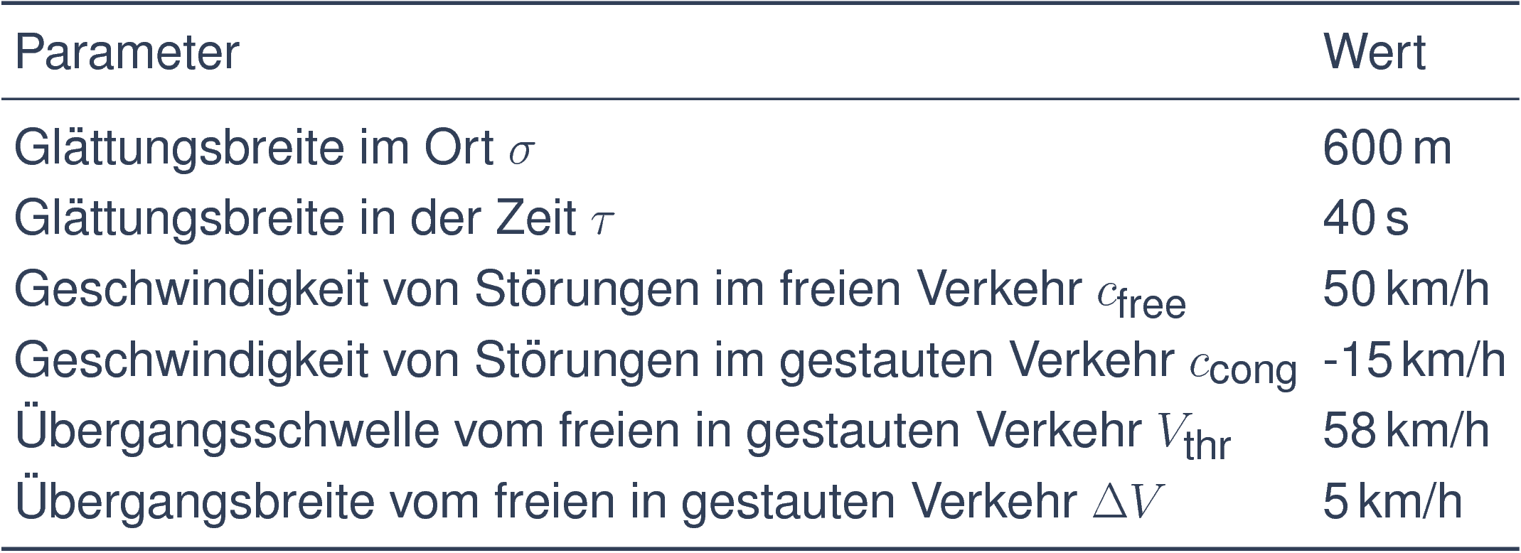
The parameters of the ASM used for generating the images of the data base are given in following table.
;)
ASM parameters
The two nonzero propagation velocities are denoted by the parameters cfree und ccong. The nonlinear speed filter is parametrized by the threshold speed Vc, and the threshold width ΔV . Furthermore, the smoothing parameters τ and σ (which only control the representation ) can be chosen in a wide range.
Calibration and Sensitivity Analysis
By variation of the parameters, we did a sensitivity analysis and tested the robustness of the adaptive soothing method with respect to the parameter settings. As reference case, we chose the speed profile of a congestion on Oct 29, 1998 on the German freeway A9-South to the north of Munich.
Sensitivity with respect to the assumed propagtion velocities
The left image of the figure below shows the speed profile after
changing the propagation velocity cfree from
its reference value 50 km/h to 200 km/h, and
ccong from its reference value -15 km/h to -10 km/h.
In the right image, we assumed cfree = 200 km/h as
well, and ccong =-20 km/h.
;)
Speed profile generated by the ASM after changing
cfree from 50 km/h to 200 km/h, and
ccong from -15 km/h to -10 km/h
;)
Speed profile of the ASM after changing
cfree from 50 km/h to 200 km/h, and
ccong from -15 km/h to -20 km/h
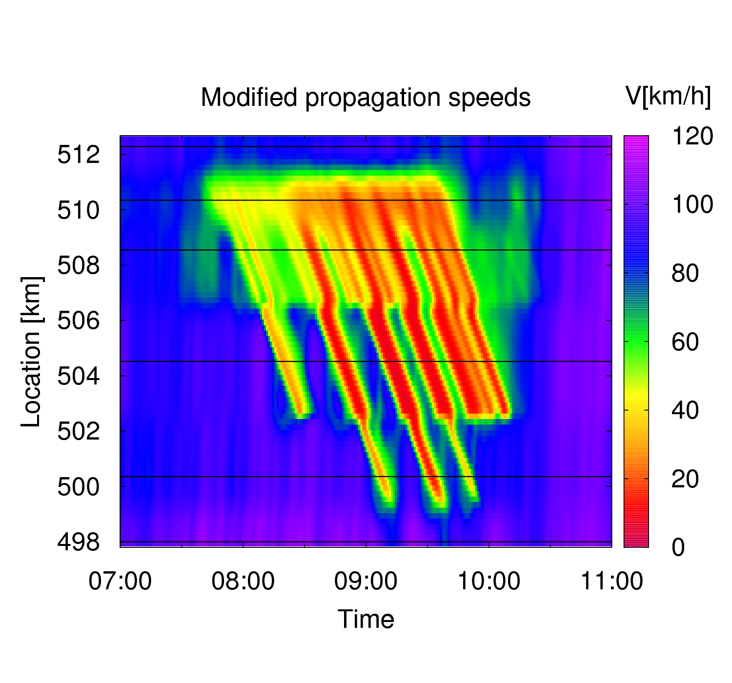
Parameters of the nonlinear speed filter
Speed profile generated by the ASM after changing Vc from 54 km/h to 40 km/h, and ΔV from 5 km/h to 20 km/h
The image on the left side shows the result of the ASM after "detuning" the parameters of the speed filter. The transition speed has been reduced by 14 km/h, while the width of the transition zone has been increased by a factor of four.
On a closer look, one recognizes that some structures has been attributed to free instead of congested traffic, a consequence of the changed transition speed which is now too low. The stop-and-go waves themselves, however, are displayed with only insignificant changes.
Of course, the sensitivity with respect to the parameters settings increases with the distance between two neighboring detector cross sections. For example, the following figure shows the result when feeding the ASM with data of only six of the nine detector cross sections.
;)
Only six detectors, changed propagation speed parameters
;)
Only six detectors, changed speed filter parameters
Result
The method turned out to be very robust, i.e., the reconstructed speed profile depends only weakly on the parameter settings, even if obviously incorrect values are assumed. Only for distances of more than 3 km between neighboring detectors (where the conventional moving averaging fails completely) one sees significant artifacts as a function of the parameter values when the parameters deviate more than 10-20% from the values in the table. The highest sensitivity is associated with the propagation speed ccong. Deviations from the calibrated value by more than 2 km/h lead to artificial steps (cf. the image to the left). For practical purpose, the reference values for freeway traffic can be assumed without further calibration. Nevertheless, the method can also be applied for the opposite problem: Estimating the propagation speeds from the data. In this case, the propagation speed is estimated by minimizing an appropriate error functional.
Validation
;)
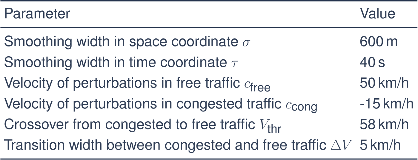
Direct plot of speed data ("ground truth") of a congestion on the British motorway M42. Here, the detectors are so dense (maximum spacing 100 m) that the data can be plotted without any data manipulation.
In spite of the obvious robustness, one cannot exclude that the logic of the ASM contains circular reasoning. After all, one input to the method is the value ccong of the propagation velocities of stop-and-go waves while the spatiotemporal pattern of the waves themselves is output of the method. Therefore, a scientific validation is necessary, i.e., a comparison of the estimated speed profile with the independently determined real situation ( "ground truth"). In order to perform such a validation, one needs a freeway section equipped with so many detectors such that the essentially complete information ( "ground truth") is already in the data. Fortunately, such sections exist. On the motorway M42 in England, the spacing between two detector cross sections is 100 m (or even less) allowing a direct plot of the data without any manipulation, see the right image (white stripes denote spatiotemporal regions with detector errors; notice that compensation of data errors is another possible application of the ASM).
;)
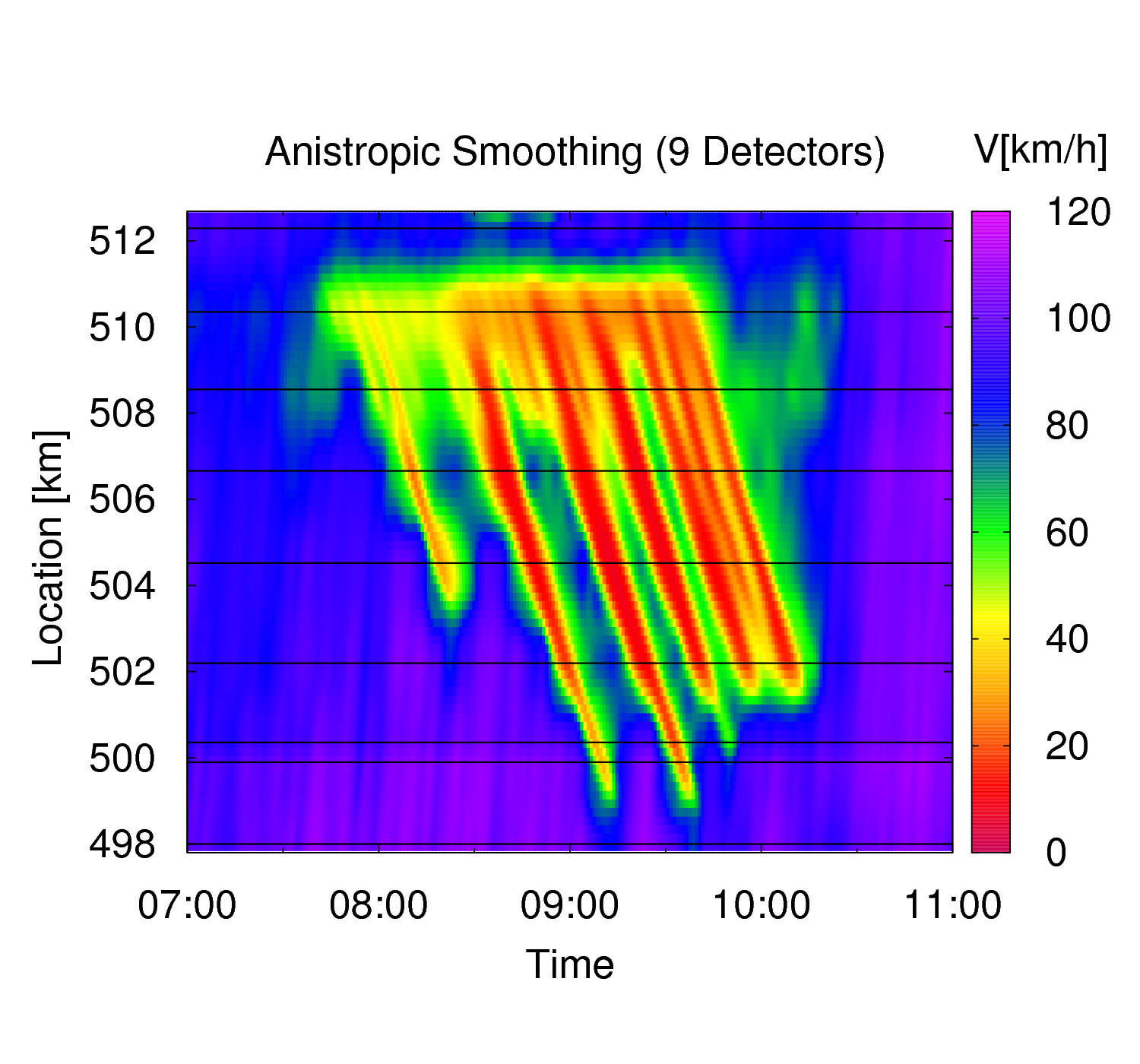
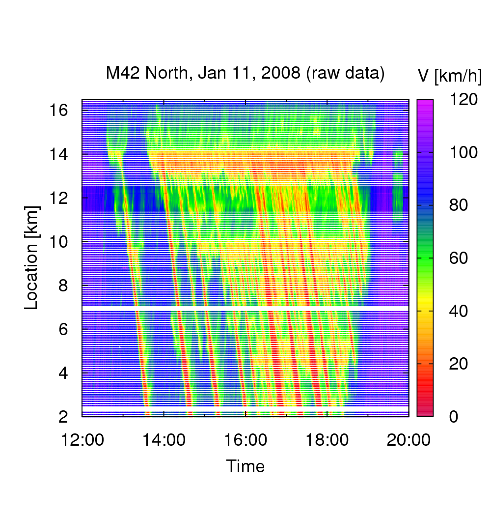
estimated traffic state derived from the ASM with reduced information: Only the data of every 10th, 20th, 30th, or 40th detector are provided.
In the validation process, the ASM is applied on an incomplete data set and the result is compared with the ground truth. The figure to the left shows the result after providing the ASM with data of every 10th, 20th, 30th, or 40th detector station corresponding to inter-detector spacings between 1 km and 4 km. We observe that the level of detail decreases with the distance between two detectors. Nevertheless, the essential features are retained up to a distance of about 3 km.
Conclusion
The adaptive smoothing method ASM allows a plausible and detailled reconstruction of the true traffic situation from stationary detectors if their distance is 3 km or less. Extensions of the ASM allow the inclusion and fusion of further point data sources such as
- Floating-Car-Data (FCD),
- Floating-Phone-Data (FPD),
- Event-oriented isolated message from authorities or private car drivers.
References
- Martin Treiber, Arne Kesting, R. Eddie Wilson:
Reconstructing the traffic state by fusion of heterogeneous data
Computer-Aided Civil and Infrastructure Engineering 26, 408-419 (2011).
Abstract,
Preprint
- Arne Kesting, Martin Treiber:
Datengestützte Analyse der Stauentstehung und -ausbreitung auf Autobahnen
Straßenverkehrstechnik Heft 01, p. 5-11 (2010).
PDF
- Martin Treiber, Dirk Helbing:
Reconstructing the spatio-temporal traffic dynamics from stationary detector data
Cooper@tive Tr@nsport@tion Dyn@mics 1 3.1-3.24.
PDF